Next: Introduction, Up: (dir) [Contents]
This document describes OpenScop, a specification of a file format and a set of data structures for polyhedral compilation tools to talk together. It also describes briefly the OpenScop Library version 0.9.0, a Free Software that provides an example of OpenScop implementation.
It would be quite kind to refer at the present document in any publication that results from the use of the OpenScop Library:
@TechReport{Bas11,
  author =      {C\'edric Bastoul},
  title =       {OpenScop: A Specification and a Library for Data
                 Exchange in Polyhedral Compilation Tools},
  month =       {September},
  year =        2011,
  institution = {Paris-Sud University, France}
}
Copyright © 2011 Paris-Sud University and INRIA.
Permission is granted to copy, distribute and/or modify this document under the terms of the GNU Free Documentation License, Version 1.2 published by the Free Software Foundation; with no Invariant Sections, with no Front-Cover Texts, and with no Back-Cover Texts. To receive a copy of the GNU Free Documentation License, write to the Free Software Foundation, Inc., 59 Temple Place, Suite 330, Boston, MA 02111-1307 USA.
| • Introduction: | ||
| • Polyhedral Representation: | ||
| • OpenScop Specification: | ||
| • OpenScop Library: | ||
| • References: |
Next: Polyhedral Representation, Previous: Top, Up: Top [Contents]
OpenScop is an open specification that defines a file format and a set of data structures to represent a static control part (SCoP for short), i.e., a program part that can be represented in the polyhedral model. The goal of OpenScop is to provide a common interface to various polyhedral compilation tools in order to simplify their interaction.
Designing a single format for tools that have different purposes (e.g., as different as code generation and data dependence analysis) may sound strange at first. However we could observe that most available polyhedral compilation tools during the last decade were manipulating more or less the same kind of data (polyhedra, affine functions...) and were actually sharing a part of their input (e.g., iteration domains and context concepts are nearly everywhere). We could also observe that those tools may rely on different internal representations, mostly based on one of the major polyhedral libraries (e.g., Polylib, PPL or isl), and this representation may change over time (e.g., when switching to a more convenient polyhedral library). The OpenScop aim is to provide a stable, unified format that offers a durable guarantee that a tool can use an output or provide an input to another tool without breaking a tool chain because of some internal changes in one element of the chain. The other promise of OpenScop is the ability to assemble or replace the basic blocks of a polyhedral compilation framework at no, or at least low engineering cost.
The policy that drives OpenScop can be summarized by these three rules:
Another, more technical, rule may be added:
The success of OpenScop in meeting its goals totally depends on its acceptance by the tool developers (that have to support it in their tools). To help them, we provide an example implementation: the OpenScop Library. This library (and in particular its API) is not part of the OpenScop specification (which includes only the file format and the set of data structures). It is licensed under the 3-clause BSD license so developers may feel free to use it in their code (either by linking it or copy-pasting its code). This document also describes this library briefly (readers are invited to read at its technical documentation). The current version of the OpenScop Library is still under evaluation, and there is no guarantee that the upward compatibility will be respected, even if we do think so. A lot of reports are necessary to freeze the library API. Thus you are very welcome and encouraged to send reports on bugs, wishes, critics, comments, suggestions or (please!) successful experiences to the OpenScop mailing list openscop-development@googlegroups.com.
This document is organized as follows. First, we provide some background on the polyhedral model and how it is used to represent and to manipulate programs (see Polyhedral Representation). Next, we describe the OpenScop specification, from the file format (see OpenScop File Format Specification) to the data structures and the OpenScop Library API (see OpenScop Data Structure Specification). Finally we will detail how to install the OpenScop Library (see Installation).
Next: OpenScop Specification, Previous: Introduction, Up: Top [Contents]
If you are reading at the OpenScop documentation, you probably don’t need any explanation about the polyhedral model. It is unlikely that someone will read this paper by mistake. However some vicious advisor may ask their poor engineers/interns/students to work for the very first time on this exciting topic. Most papers on polyhedral compilation are hard to read. Despite my efforts, mine are no exception according to some reviewers. Hence I give there a new try to provide a comprehensive explanation of the polyhedral model without the size and style limits of a classical research paper.
Be aware that to be able to understand the polyhedral model, there are a few prerequisites. You should not read the following while you still ignore what is:
for loop construction in C programs (do loops in FORTRAN are OK too!),
If you do not know those concepts, please do some search and come back afterwards. And if you are courageous enough, send me a few lines that describe them so I can insert them here!
| • Motivation: | ||
| • Thinking in Polyhedra: | ||
| • What's Next?: |
Next: Thinking in Polyhedra, Up: Polyhedral Representation [Contents]
A direct translation of high level programs written, e.g., in C, to assembly then to object code is likely to produce (very) inefficient applications. Architectures are quite complex, including several levels of cache memory, many cores, deep pipelines, various number of functional units, of registers etc. The list of such "architectural features" is growing with each new generation of processors. To achieve the best performance, the object program must use these features in a smart way. Programmers use high level languages for productivity and portability: typically they do not have to take care of the target architecture but to ensure they write programs which produce the right output. Hence, the problem of mapping the program to the target architecture in the most efficient way is left to the compiler.
The compiler may see a high level program as a specification of an output. The program is a list of instructions to be executed to produce the output. As long as the output is guaranteed to be as the programmer specified in his code, the compiler is free to modify the program. For instance, let us imagine we are working on an architecture with only three registers and we consider the following statements written by a programmer:
x = a + b;
y = c + d;
z = a * b;
It is easy to see that we can reorder the three statements in any way without
modifying the semantics (no statement reads or writes a variable that another
statement writes). Because of the lack of registers, the solutions such that
the first and the third statements are one after the other are better
because a and b will be put in the processor registers by
one statement and can be reused directly by the other one
without reading from memory (this is called a data locality
improving transformation). Hence a better statement order is, e.g.:
x = a + b;
z = a * b; // a and b are still in processor registers
y = c + d;
We can also notice that it is possible to run the three statements in parallel (possibly on different processors). The programmer may explicit this in a way the compiler and/or the architecture is able to understand. For instance, we can use OpenMP to describe parallelism (this is called a parallelizing transformation):
#pragma omp parallel sections
{
   #pragma omp section
   {
     x = a + b;
   }
   #pragma omp section
   {
     y = c + d;
   }
   #pragma omp section
   {
     z = a * b;
   }
}
However, the right way to optimize this program is probably a tradeoff between these two techniques. This is true if, e.g., the target architecture has some limitations to run too many operations in parallel, or, like in our case, when some data may be reused by some processors. Hence, the best optimization for our small example is probably the following:
#pragma omp parallel sections
{
   #pragma omp section
   {
     x = a + b;
     z = a * b;
   }
   #pragma omp section
   {
     y = c + d;
   }
}
This example is quite trivial because the statements are executed only once. The real sport begins when we have to deal with loops, as we will see momentarily. However, polyhedral compilation framework users have to be conscious that we need to transform programs to achieve the best performance and that the best transformation that has to be discovered (at the price of many, many efforts) and performed may be quite complex. Hence the need of powerful model and tools.
Next: What's Next?, Previous: Motivation, Up: Polyhedral Representation [Contents]
Since the very first compilers, the internal representation of programs is the Abstract Syntax Tree, or AST. In such representation, each statement appears only once even if it is executed many times (e.g., when it is enclosed inside a loop). This is a limitation for finding and applying complex transformations:
The Polyhedral Model is a convenient alternative representation which combines analysis power, expressiveness and high flexibility. The drawback is it breaks the classical structure of programs that every programmer is familiar with. It requires some (real) efforts to be smoothly manipulated, but it definitely worth it. It is based on three main concepts, iteration domain, scattering function and access function that are described in depth in the following sections.
A program part that can be represented using the Polyhedral Model is called a Static Control Part or SCoP for short.
| • Iteration Domain: | ||
| • Scattering Function: | ||
| • Access Function: |
Next: Scattering Function, Up: Thinking in Polyhedra [Contents]
The key aspect of the polyhedral model is to consider statement
instances. A statement instance is one execution of a statement.
A statement
outside a loop has only one instance while those inside loops may have many.
Let us consider the following code with two statements S1
and S2:
pi = 3.14;               // S1
for (i = 0; i < 5; i++)
  A[i] = pi;             // S2
The list of statement instances is the following (we just have to fully unroll the loop):
pi = 3.14;
A[0] = pi;
A[1] = pi;
A[2] = pi;
A[3] = pi;
A[4] = pi;
Each instance of a statement which is enclosed inside a loop may be referred
thanks to its outer loop counters (or iterators). In the polyhedral
model we consider statements as functions of the outer loop counters that may
produce statement instances:
instead of simply "S2", we use preferably the notation S2(i).
For instance we denote the statement instance A[3] = pi; of the
previous example as S2(3). This means instance of
statement S2 for i = 3.
If a statement S3 is enclosed inside two loops of iterators i
(outermost loop) and j (innermost loop), we would denote it
S3(i,j), and so on with more enclosing loops.
The ordered list
of iterators (ordered from the outermost iterator to the innermost iterator)
is called the iteration vector. For instance the iteration vector for
S3 is (i,j), for S2 it is (i), and for S1
it is empty since it has no enclosing loop: (). A more precise reading
at the notation S2(3) would show that it denotes the instance of
statement S2 for the iteration vector (2).
Obviously, dealing with statement instances does not mean we have to unroll all
loops. First because there would be probably too many instances to deal with,
and second because we probably just do not know how many instances there are.
For instance in the following loop it is impossible to know (at compile time)
how many times the statement S3 will be executed:
for (i = 2; i <= N; i++)
  for (j = 2; j <= N; j++)
    A[i] = pi;             // S3
Such a loop is said to be parametric: it depends on
(at least) a value called a parameter which is not modified
during the execution of the whole loop, but is unknown at compile time.
Here, the only parameter is N.
A compact way to represent all the instances of a given statement
is to consider the set of all possible values of its iteration vector.
This set is called the iteration domain. It can be conveniently
described thanks to all the constraints on the various iterators the statement
depends on. For instance, let us consider
the statement S3 of the previous program. The iteration domain is the set
of iteration vectors (i,j). Because of the parameter, we are not able to
achieve a precise list of all possible values. It would look like this:
(2,2)  (2,3)  (2,4)  ...  (2,N)
(3,2)  (3,3)  (3,4)  ...  (3,N)
...    ...    ...    ...  ...
(N,2)  (N,3)  (N,4)  ...  (N,N)
A better way is to say it is the set
of iteration vectors (i,j) such that i is an integer greater or
equal than 2 and lower or equal than N, and j is an integer
greater or equal than 2 and lower or equal than N. This may be written
in the following mathematical form:
D_S3 = {(i,j) in Z^2 | 2 <= i <= N && 2 <= j <= N }
It is easy to see that this iteration domain is a part of the 2-dimensional space
Z^2.
We often use in our research papers a graphical representation that gives a better view of this subspace:
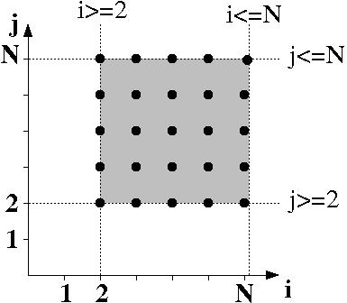
Here, the iteration domain is specified thanks to a set of constraints. When those constraints are affine and depend only on the outer loop counters and some parameters, the set of constraints defines a polyhedron (more precisely this is a Z-polyhedron, but we use polyhedron for short). Hence the polyhedral model!
To manipulate a set of affine constraints easily, we rely on a matrix
representation. To write it, we use the homogeneous iteration vector:
it is simply the iteration vector with some additional dimensions to
represent the parameters and the constant.
For instance for the statement S3, the
iteration vector in homogeneous coordinates is (i, j, N, 1)
(we will now call it iteration vector directly for short).
Then we write all the constraints as affine inequalities of the form
affine constraint
>= 0.
For instance for the statement S3 the set of constraints is:
    i - 2 >= 0
   -i + N >= 0
    j - 2 >= 0
   -j + N >= 0
Lastly, we translate the constraint system to the form
domain matrix * iteration vector >= 0:
[  1  0  0 -2 ]   [ i ]    [ 0 ]
[ -1  0  1  0 ]   [ j ]    [ 0 ]
[  0  1  0 -2 ] * [ N ] >= [ 0 ]
[  0 -1  1  0 ]   [ 1 ]    [ 0 ]
The domain matrix will be used in all our tools to provide the information on the iteration domain of a given statement (the iteration vector is in general an implicit information).
Next: Access Function, Previous: Iteration Domain, Up: Thinking in Polyhedra [Contents]
There is no ordering information inside the iteration domain: it only describes the set of statement instances but not the order in which they have to be executed relatively to each other. In the past the lexicographic order of the iteration domain was considered, this is no more true (especially when using CLooG). If we do not provide any ordering information, this means that the statement instances may be executed in any order (this is useful, e.g., to specify parallelism). However, some statement instances may depend on some others and it may be critical to enforce a given order (or non-order). Hence we need another information.
We call scattering any kind of ordering information in the polyhedral model. There exists many kind of ordering, such as allocation, scheduling, chunking etc. They are all expressed in the same way, i.e., using logical stamps, but they may have different semantics.
In the case of scheduling, the logical stamps are logical dates that express at which date a statement instance has to be executed. For instance, let us consider the following three statements:
x = a + b;   // S1
y = c + d;   // S2
z = a * b;   // S3
The scheduling of a statement S is typically
denoted by
T_S.
Let us consider the following logical dates for each statement:
T_S1 = 1
T_S2 = 2
T_S3 = 3
It means that statement S3 has to be executed at logical date
1, statement S1 has to be executed at logical date
2 and statement S2 has to be executed at logical date
3. The target code has to respect this scheduling (the order of
the logical dates), hence it would look like the following where the
variable t denotes the time:
t = 1;
z = a * b;   // S3
t = 2;
x = a + b;   // S1
t = 3;
y = c + d;   // S2
When some statements share the same logical date, this means that, once the program reaches this logical date, the two statements can be executed in any order, or better, in parallel. For instance let us consider the following scheduling:
T_S1 = 1
T_S2 = 2
T_S3 = 1
Statements S1 and S3 have the same logical date,
moreover, S2 has a greater logical date than S1 and S3.
Hence the target code would be:
t = 1;
#pragma omp parallel sections
{
   #pragma omp section
   {
     x = a + b;   // S1
   }
   #pragma omp section
   {
     z = a * b;   // S3
   }
}
t = 2;
y = c + d;        // S2
Logical dates may be multidimensional, as clocks: the first dimension may correspond to days (most significant), the next one to hours (less significant), the third to minutes and so on. For instance we can consider the following multidimensional schedules for our example:
T_S1 = (1,1)
T_S2 = (2,1)
T_S3 = (1,2)
It is not very hard to decypher the meaning of such scheduling.
Because of the first dimension, statements S1 and S3 will be
executed before statement S2 (S1 and S3 are executed at
day 1, while S2 is executed at day 2). The second dimension is not
really useful there for S2 because it is the only statement executed
at day 2. Nevertheless it allows to order S1 and
S3 relatively to each other since S1 is executed at hour 1 of day
1 while S3 is executed at hour 2 of day 1.
The corresponding target code is the following, with some
additional time variables for a better view of the ordering (t1
corresponds to the first time dimension, t2 to the second one):
t1 = 1;
t2 = 1;
x = a + b;   // S1
t2 = 2;
z = a * b;   // S3
t1 = 2;
t2 = 1;
y = c + d;   // S2
In the case of allocation (in the literature we can find some
papers calling it placement), the logical stamp is a processor
number expressing on which processor a statement instance has to be
executed. Typically, allocations are written in the same way as scheduling.
Here, we denote it P_S for a statement S.
For instance, let us consider the following allocation:
P_S1 = 1
P_S2 = 2
P_S3 = 1
The corresponding target code has to take into account that both
statements S1 and S3 have to be executed on the same processor
(they have the same logical number 1) and that statement S2 has
to be executed on another processor (logical number 2). A possible target code
is the following:
#pragma omp parallel sections
{
   #pragma omp section
   {
     // Logical processor 1
     x = a + b;   // S1
     z = a * b;   // S3
   }
   #pragma omp section
   {
     // Logical processor 2
     y = c + d;   // S2
   }
}
We can note that no order has been specified for the
statements S1 and S3 that are executed on the same processor.
Hence any order is satisfying. For sake of flexibility, it is usual to build
a scattering whose various dimensions do not have the same semantics. A
typical construction is space/time mapping where the first n
dimensions are devoted to allocation, then the last m
dimensions are devoted to scheduling. Typically, space/time mapping is
written in the same way as scheduling.
Here we denote it M_S for a statement S.
For instance, let us consider the following space/time mapping for our
example where one dimension is devoted to mapping and one dimension is
devoted to scheduling:
M_S1 = (1,2)
M_S2 = (2,1)
M_S3 = (1,1)
Here we have the same first dimension as the previous example, thus
the allocation of the statements to processors is the same. The second
dimension precises on a given processor at which logical date a statement
instance has to be executed. Here, the statement S1 is executed at
day 2 on processor 1 while the statement S3 is executed at day 1 onto
the same processor. It follows this space/time mapping corresponds to the
following target code (we added an additional variable to represent the
local logical clocks):
#pragma omp parallel sections
{
   #pragma omp section
   {
     // Logical processor 1
     t = 1;
     z = a * b;   // S3
     t = 2;
     x = a + b;   // S1
   }
   #pragma omp section
   {
     // Logical processor 2
     t = 1;
     y = c + d;   // S2
   }
}
For the same reason as discussed for iteration domains (see Iteration Domain), it is not possible to define a scattering for each statement instance, especially if the statement belongs to a (possibly parametric) loop. The iteration vector fully defines an instance of a given statement. Thus, a practical way to provide a scattering for each instance of a given statement is to use a function that depends on the iteration vector. In this way the function may associate to each iteration vector a different scattering. We call these functions scattering functions. Scattering functions are affine functions of the outer loop counter and the global parameters. For instance, let us consider the following source code:
for (i = 2; i <= 4; i++)
  for (j = 2; j <= 4; j++)
    P[i+j] += A[i] + B[j]; // S4
The iteration domain of the statement S4 is:
D_S4= {(i,j) in Z^2 | 2 <= i <= 4 && 2 <= j <= 4 }.
If you are still not comfortable with the mathematical notation, it corresponds to the following graphical representation:
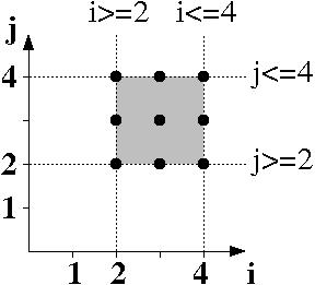
The list of the statement instances of S4 (the integer
points of its iteration domain) corresponds to the following iteration vectors:
iteration vector
     (2,2)
     (2,3)
     (2,4)
     (3,2)
     (3,3)
     (3,4)
     (4,2)
     (4,3)
     (4,4)
Let us suppose we want to schedule the instances of the statement
S4 (the integer points of its iteration domain) using the following
scheduling function:
T_S4(i,j) = (j+2,3*i+j)
We only need to apply the function to each iteration vector to find the logical date of each instance:
iteration vector       logical date
     (2,2)       -->       (4,8)
     (2,3)       -->       (5,9)
     (2,4)       -->       (6,10)
     (3,2)       -->       (4,11)
     (3,3)       -->       (5,12)
     (3,4)       -->       (6,13)
     (4,2)       -->       (4,14)
     (4,3)       -->       (5,15)
     (4,4)       -->       (6,16)
The polyhedral model users do not have to take care about the generation of a
target code that respects the scattering: the
CLooG1 tool is there to
solve the problem quite easily. For the previous
example, the target code would be the following (t1 and t2
correspond to the two dimensions of the logical date, the reader may
take care that this code actually implements the scattering function):
for (t1 = 4; t1 <= 6; t1++) {
  for (t2 = t1+4; t2 <= t1+10; t2++) {
    if ((-t1+t2+2)%3 == 0) {
      i = (-t1+t2+2)/3 ;
      j = t1-2 ;
      P[i+j] += A[i] + B[j]; // S4
    }
  }
}
Obviously with such a twisted scheduling, it is hard to see the "meaning" of the transformation. To name any kind of program transformation as a magic spell ("tile", "fuse", "skew"...) is an old bad habit which is not relevant anymore in the polyhedral model: a scheduling may be an arbitrary complex sequence of basic-old-good transformations. Nevertheless it is most of the time quite easy to translate well known transformations to schedules. For instance, let us consider this new scheduling function:
T_S4(i,j) = (j,i)
Using CLooG, we can generate the target code:
for (t1 = 2; t1 <= 4; t1++) {
  for (t2 = 2; t2 <= 4; t2++) {
    i = t2;
    j = t1;
    P[i+j] += A[i] + B[j]; // S4
  }
}
It is easy to see (and analyze) that it corresponds to a classical loop interchange transformation.
A very useful example of multi-dimensional scattering functions is the scheduling of the original program. The method to compute it is quite simple (see Fea92). The idea is to build an abstract syntax tree of the program and to read the scheduling for each statement. For instance, let us consider the following implementation of a Cholesky factorization:
/* A Cholesky factorization kernel. */
for (i=1;i<=N;i++) {
  for (j=1;j<=i-1;j++) {
    a[i][i] -= a[i][j] ;           // S1
  }
  a[i][i] = sqrt(a[i][i]) ;        // S2
  for (j=i+1;j<=N;j++) {
    for (k=1;k<=i-1;k++) {
      a[j][i] -= a[j][k]*a[i][k] ; // S3
    }
    a[j][i] /= a[i][i] ;           // S4
    }
  }
}
The corresponding abstract syntax tree is shown in the following figure. It directly gives the scattering functions (schedules) for all the statements of the program (just follow the paths).
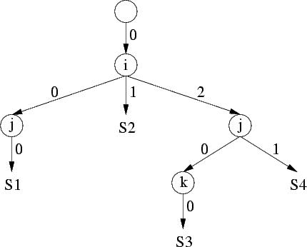
T_S1(i,j)   = (0,i,0,j,0)
T_S2(i)     = (0,i,1)
T_S3(i,j,k) = (0,i,2,j,0,k,0)
T_S4(i,j)   = (0,i,2,j,1)
These schedules depend on the iterators and give for each instance of each statement a unique execution date. Using such scattering functions allows CLooG to re-generate the input code.
To easily manipulate the scattering function of any
statement S, we translate it to the matrix form:
T_S(iteration vector)
= scattering matrix * iteration vector.
For instance let us consider again our previous example
T_S4(i,j) = (j+2,3*i+j).
We write it in the following way:
     [ i ]    [  0  1  2 ]   [ i ]
T_S4([ j ]) = [  3  1  0 ] * [ j ]
     [ 1 ]                   [ 1 ]
The scattering matrix will be used in all our tools to provide the information on the scattering of a given statement (the iteration vector is in general an implicit information).
Previous: Scattering Function, Up: Thinking in Polyhedra [Contents]
Before applying any transformation, it is essential to deeply analyze both the original program and the transformation to ensure the transformation does not imply any modification of the original program semantics. In the polyhedral model, we are able to achieve an exact analysis when all the memory accesses are made through arrays (note that variables are a particular case of arrays since they are simply arrays with only one memory location) with affine subscripts that depend on outer loop counters and global parameters (note that subscripts are sometimes called index or accesses in the literature).
For instance let us consider the array access A[2*i+j][j][i+N]. It has
three dimensions, each subscript dimension is an affine form of some outer loop
iterarors (i and j) and global parameters (N) hence
it corresponds to an acceptable array access to be analyzed in the
polyhedral model.
Each array access can target a different memory cell depending on the statement instance, i.e., depending on the iteration vector. Thus we use access functions (or subscript functions, or index functions, as you prefer to call it) depending on the iteration vector to describe an array access. In our example, the access function would be written F_A(i, j) = (2*i+j, j, i+N).
To easily manipulate the access function of any
array A, we translate it to the matrix form:
F_A(iteration vector)
= access matrix * iteration vector.
For instance let us consider again our previous example. We would
write it in the following way:
    [ i ]    [  2  1  0  0 ]   [ i ]
F_A([ j ]) = [  0  1  0  0 ] * [ j ]
    [ N ]    [  1  0  1  0 ]   [ N ]
    [ 1 ]                      [ 1 ]
The access matrix will be used in all our tools to provide the information on the access of a given statement (the iteration vector is in general an implicit information).
Previous: Thinking in Polyhedra, Up: Polyhedral Representation [Contents]
OK, now you have an idea about how we do represent a program part in the polyhedral model. You know the three main concepts, namely: domain, scattering and access. What can you do with this?! Well, pretty much anything related to code restructuring! The core idea will be to rely on the mathematical representation to extract useful information about your code (data reuse, parallelism...) and to generate a scattering to benefit from the properties you analysed. However, OpenScop’s documentation is not the right place to learn at this (OpenScop is all about representation, not about manipulation). Probably it is the right time for you to have a look at:
Have fun :-) !
Next: OpenScop Library, Previous: Polyhedral Representation, Up: Top [Contents]
OpenScop provides an explicit polyhedral representation of a static control part. It has been designed by various polyhedral compilation tool writers from various institutions. It builds on previous popular polyhedral file and data structure formats (such as .cloog and CLooG data structures) to provide a unique, extensible format to most polyhedral compilation tools. It is composed of two parts. The first part, the so-called core part, is devoted to the polyhedral representation of a SCoP. It contains what is strictly necessary to build a complete source-to-source framework in the polyhedral model and to output a semantically equivalent code for the SCoP, from analysis to code generation. The second part of the format, the so-called extension part, contains extensions to provide additional informations to some tools.
| • Preliminary Example: | ||
| • OpenScop File Format Specification: | ||
| • OpenScop Data Structure Specification: | ||
| • Extensions: | ||
| • History: |
OpenScop is a specification for representing static control program parts in the polyhedral model. Thus, we can translate some code parts to an equivalent OpenScop representation. As an example, let us consider the following matrix-multiply kernel:
#pragma scop
if (N > 0) {
  for (i = 0; i < N; i++) {
    for (j = 0; j < N; j++) {
      C[i][j] = 0.0;
      for (k = 0; k < N; k++)
        C[i][j] = C[i][j] + A[i][k] * B[k][j];
    }
  }
}
The Clan2
tool may be used to translate this code part to an OpenScop
representation automatically. The #pragma scop is used here for
Clan, but some other tool may not need it. Here is the result of the
translation to an OpenScop textual representation.
Explanations will follow and it is not as cryptic as it seems to be !
<OpenScop>

# =============================================== Global
# Backend Language
C

# Context
CONTEXT
1 3 0 0 0 1
# e/i | N  | 1
   1    1   -1    ## N-1 >= 0

# Parameter names are provided
1
# Parameter names
<strings>
N
</strings>

# Number of statements
2

# =============================================== Statement 1
# Number of relations describing the statement
3

# ----------------------------------------------  1.1 Domain
DOMAIN
4 5 2 0 0 1
# e/i | i    j  | N  | 1
   1    1    0    0    0    ## i >= 0
   1   -1    0    1   -1    ## -i+N-1 >= 0
   1    0    1    0    0    ## j >= 0
   1    0   -1    1   -1    ## -j+N-1 >= 0

# ----------------------------------------------  1.2 Scattering
SCATTERING
5 10 5 2 0 1
# e/i| s1   s2   s3   s4   s5  | i    j  | N  | 1
   0   -1    0    0    0    0    0    0    0    0    ## s1 = 0
   0    0   -1    0    0    0    1    0    0    0    ## s2 = i
   0    0    0   -1    0    0    0    0    0    0    ## s3 = 0
   0    0    0    0   -1    0    0    1    0    0    ## s4 = j
   0    0    0    0    0   -1    0    0    0    0    ## s5 = 0

# ----------------------------------------------  1.3 Access
WRITE
3 8 3 2 0 1
# e/i| Arr  [1]  [2] | i    j  | N  | 1
   0   -1    0    0    0    0    0    1    ## C
   0    0   -1    0    1    0    0    0    ##  [i]
   0    0    0   -1    0    1    0    0    ##     [j]

# ----------------------------------------------  1.4 Statement Extensions
# Number of Statement Extensions
1
<body>
# Number of original iterators
2
# Original iterator names
i j
# Statement body expression
C[i][j] = 0.0;
</body>

# =============================================== Statement 2
# Number of relations describing the statement
5

# ----------------------------------------------  2.1 Domain
DOMAIN
6 6 3 0 0 1
# e/i|  i    j    k  | N  | 1
   1    1    0    0    0    0    ## i >= 0
   1   -1    0    0    1   -1    ## -i+N-1 >= 0
   1    0    1    0    0    0    ## j >= 0
   1    0   -1    0    1   -1    ## -j+N-1 >= 0
   1    0    0    1    0    0    ## k >= 0
   1    0    0   -1    1   -1    ## -k+N-1 >= 0

# ----------------------------------------------  2.2 Scattering
SCATTERING
7 13 7 3 0 1
# e/i| s1   s2   s3   s4   s5   s6   s7  | i    j    k  | N  | 1
   0   -1    0    0    0    0    0    0    0    0    0    0    0   ## s1 = 0
   0    0   -1    0    0    0    0    0    1    0    0    0    0   ## s2 = i
   0    0    0   -1    0    0    0    0    0    0    0    0    0   ## s3 = 0
   0    0    0    0   -1    0    0    0    0    1    0    0    0   ## s4 = j
   0    0    0    0    0   -1    0    0    0    0    0    0    1   ## s5 = 1
   0    0    0    0    0    0   -1    0    0    0    1    0    0   ## s6 = k
   0    0    0    0    0    0    0   -1    0    0    0    0    0   ## s7 = 0

# ----------------------------------------------  2.3 Access
WRITE
3 9 3 3 0 1
# e/i| Arr  [1]  [2] | i    j    k  | N  | 1
   0   -1    0    0    0    0    0    0    1    ## C
   0    0   -1    0    1    0    0    0    0    ##  [i]
   0    0    0   -1    0    1    0    0    0    ##     [j]

READ
3 9 3 3 0 1
# e/i| Arr  [1]  [2] | i    j    k  | N  | 1
   0   -1    0    0    0    0    0    0    1    ## C
   0    0   -1    0    1    0    0    0    0    ##  [i]
   0    0    0   -1    0    1    0    0    0    ##     [j]

READ
3 9 3 3 0 1
# e/i| Arr  [1]  [2] | i    j    k  | N  | 1
   0   -1    0    0    0    0    0    0    2    ## A
   0    0   -1    0    1    0    0    0    0    ##  [i]
   0    0    0   -1    0    0    1    0    0    ##     [k]

READ
3 9 3 3 0 1
# e/i| Arr  [1]  [2] | i    j    k  | N  | 1
   0   -1    0    0    0    0    0    0    3    ## B
   0    0   -1    0    0    0    1    0    0    ##  [k]
   0    0    0   -1    0    1    0    0    0    ##     [j]

# ----------------------------------------------  1.4 Statement Extensions
# Number of Statement Extensions
1
<body>
# Number of original iterators
3
# Original iterator names
i j k
# Statement body expression
C[i][j] = C[i][j] + A[i][k] * B[k][j];
</body>

# =============================================== Extensions
<comment>
May the power of the polyhedral model be with you.
</comment>

</OpenScop>
We will not describe here precisely the structure and the components of this output, this is described in depth in a further section (see OpenScop File Format Specification). This format has been designed to be a possible input or output file format of most of polyhedral compilation tools. If you read the description of the polyhedral representation of programs, you should already feel familiar with this file format (see Polyhedral Representation).
Next: OpenScop Data Structure Specification, Previous: Preliminary Example, Up: OpenScop Specification [Contents]
| • Relations: | ||
| • Generics: |
The following grammar describes the structure of the OpenScop file format where terminals are preceeded by "_". Except stated otherwise, there can be at most one terminal per line in the file. Moreover, each line may finish with a comment, starting by the ‘#’ character. Each relevant part will be explained in more details momentarily:
OpenScop              ::= Start_tag Data End_tag
Start_tag             ::= "<OpenScop>"
End_tag               ::= "</OpenScop>"
Data                  ::= Context Statements Extension_list
Context               ::= Language Parameter_Domain Parameters
Statements            ::= Nb_statements Statement_list
Statement_list        ::= Statement Statement_list | (void)
Relation_list         ::= _Relation Relation_list  | (void)
Extension_list        ::= _Generic  Extension_list | (void)
Statement             ::= Statement_relations Statement_extensions
Statement_extensions  ::= Num_Extensions Extension_list
Parameters            ::= "0" | "1" Parameter_information
Statement_relations   ::= Nb_relations Relation_List
Parameter_domain      ::= _Relation
Language              ::= _String
Nb_Relations          ::= _Integer
Num_extensions        ::= _Integer
Parameter_information ::= _Generic
The ‘Context’ and the ‘Statements’ parts compose the core part, i.e., what is strictly necessary to build a complete source to source framework based on OpenSCop:
strings
(see Strings Generic) for instance.
body
(see Body Generic) for instance.
The ‘Extension_list’ represents the extension part and may contain an arbitrary number of generic informations (see Generics). Few examples of possible extensions are presented in a further section (see Extensions).
As shown by the grammar, the input file describes the various pieces of information based on strings, integers, relations and generics. Relations and Generics are specific to OpenScop and are described in depth in the following Sections (see Relations and see Generics).
Next: Generics, Up: OpenScop File Format Specification [Contents]
| • Iteration Domain Relation: | ||
| • Context Domain Relation: | ||
| • Scattering Relation: | ||
| • Access Relation: |
Relations are the essence of the OpenScop format and contain the "polyhedral" information. They are used to describe either an iteration domain, or a context domain, or a scattering or a memory access.
We use the relation term as a shortcut to denote a union of convex relations, each element of the union being described by a set of constraints in an extended PolyLib format (see Wil93). The number of elements in the union is given by an integer on the first line, optionally followed by a comment starting with ‘#’. This number of elements can be omitted when there is only one element. Each element in the union has the following syntax:
UNDEFINED: generic relation,
CONTEXT: for context information,
DOMAIN: for iteration domains,
SCATTERING: for scattering relation,
READ: for read accesses,
WRITE: for write accesses,
MAY_WRITE: for may-write accesses,
The sum of the last four numbers should be equal to the number of columns minus two. The remaining two columns are the equality/inequality indicator and the constant term. The number of parameters should be the same for all relations in the entire OpenScop file or data structure.
This representation is the basis for several purposes. Examples for iteration domains (see Iteration Domain Relation), context domains (see Context Domain Relation), scattering relations (see Scattering Relation) and access relations (see Access Relation) are provided in further sections.
Next: Context Domain Relation, Up: Relations [Contents]
Iteration domain represents the set of instances of the corresponding statement. OpenScop iteration domains are represented as relations with the following conventions:
DOMAIN,
For instance, assuming that ‘i’, ‘j’ and ‘k’ are the loop iterators and ‘M’ and ‘N’ are the parameters, the domain defined by the following constraints :
   -i + M >= 0
   -j + N >= 0
i + j - k >= 0
can be written in the input file as follows:
# This is an iteration domain
DOMAIN
1 # Number of relations in the union
3 7 3 0 0 2                  # 3 rows, 7 cols: 3 output dims and 2 params
# e/i| i   j   k | M   N | 1
   1  -1   0   0   1   0   0 #    -i + M >= 0
   1   0  -1   0   0   1   0 #    -j + N >= 0
   1   1   1  -1   0   0   0 # i + j - k >= 0
Equivalently, it can be written in the following way as the number of relations in the union can be omitted if it is 1:
# This is an iteration domain
DOMAIN
3 7 3 0 0 2                  # 3 rows, 7 cols: 3 output dims and 2 params
# e/i| i   j   k | M   N | 1
   1  -1   0   0   1   0   0 #    -i + M >= 0
   1   0  -1   0   0   1   0 #    -j + N >= 0
   1   1   1  -1   0   0   0 # i + j - k >= 0
As an example for unions, let us consider the following pseudo-code:
for (i = 1; i <= N; i++) {
  if ((i >= M) || (i <= 2*M))
    S1(i);
}
The iteration domain of ‘S1’ can be divided into two relations and written in the OpenScop file as follows:
# This is an iteration domain
DOMAIN
2 # Number of relations in the union
# Union part No.1
3 5 1 0 0 2          # 3 rows, 5 cols: 1 output dim and 2 params
# e/i| i | M   N | 1
   1   1   0   0  -1 #  i >= 1
   1  -1   0   1   0 #  i <= N
   1   1  -1   0   0 #  i >= M
# Union part No.2
3 5 1 0 0 2          # 3 rows, 5 cols: 1 output dim and 2 params
# e/i| i | M   N | 1
   1   1   0   0  -1 #  i >= 1
   1  -1   0   1   0 #  i <= N
   1  -1   2   0   0 #  i <= 2*M
As an example for local dimensions (existentially quantified dimensions), let us consider the following pseudo-code:
for (i = 1; i <= N; i++) {
  if ((i % 2) == 0)
    S1(i);
}
The iteration domain of ‘S1’ is composed of all even integer values between 1 and N. The "divisible by two" constraint can be expressed as follows: there exists an integer ‘ld’ such that ‘i = 2*ld’. We encode this thanks to a new local dimension:
# This is an iteration domain
DOMAIN
3 5 1 0 1 1          # 3 rows, 5 cols: 1 output dim, 1 local dim, 1 param
# e/i| i |ld | N | 1
   0   1  -2   0   0 #  i = 2*ld
   1   1   0   0   1 #  i >= 1
   1  -1   0   1   0 #  i <= N
Next: Scattering Relation, Previous: Iteration Domain Relation, Up: Relations [Contents]
The context domain is a particular case of iteration domain (see Iteration Domain Relation) where there are only constraints about parameters (no loop iterators). Hence it is the same as an iteration domain, with the following conventions:
CONTEXT,
Next: Access Relation, Previous: Context Domain Relation, Up: Relations [Contents]
Scattering relation maps an iteration domain to a logical time and/or space (and/or) anything. OpenScop scattering information is represented as relations (see Relations) with the following conventions:
SCATTERING,
As an example of a scattering relation and assuming that ‘i’, ‘j’ and ‘k’ are the loop iterators and ‘M’ and ‘N’ are the parameters, take for instance:
T_{S}(i,j,k) = (j+2,3*i+j,k+N+1).
We can represent it in the following way:
# A scattering relation
SCATTERING
# 3 rows, 10 columns: 3 scattering dimensions, 3 iterators, 2 parameters
3 10 3 3 0 2
# e/i|s1  s2  s3 | i   j   k | M   N | 1
   0  -1   0   0   0   1   0   0   0   2 # s1 = j+2
   0   0  -1   0   3   1   0   0   0   0 # s2 = 3*i+j
   0   0   0  -1   0   0   1   0   1   1 # s3 = k+N+1
Previous: Scattering Relation, Up: Relations [Contents]
Access relation maps an iteration domain to an array space. Each array accessed in the SCoP has a unique identification number. OpenScop relation information is represented as relations (see Relations) with the following conventions:
READ, for read accesses,
WRITE, for write accesses,
MAY_WRITE, for may write accesses,
As an example of a scattering relation and
assuming that ‘i’, ‘j’ and ‘k’ are the loop
iterators and ‘M’ and ‘N’ are the parameters, let us consider
the array access A[2*i+j][j][i+N] (the identifier of A is 42),
and let us suppose this is a read access. Its representation would be the
following:
# A read access relation
READ
# 4 rows, 11 columns: 4 array dimensions, 3 iterators, 2 parameters
4 11 4 3 0 2
# e/i|Arr [1] [2] [3]| i   j   k | M   N | 1
   0  -1   0   0   0   0   0   0   0   0  42   # A
   0   0  -1   0   0   2   1   0   0   0   0   #  [2*i+j]
   0   0   0  -1   0   0   1   0   0   0   0   #         [j]
   0   0   0   0  -1   1   0   0   0   1   0   #            [i+N]
To understand this representation, consider that OpenScop accesses
are general memory accesses and not array accesses. The memory is
seen as a big array Mem while usual array names correspond to
the first dimension. Hence our example translates to Mem[42][2*i+j][j][i+N].
Unions of access relations are allowed. In this case, each union part must refer at the same array identifier, and the number of dimensions must be consistent.
Previous: Relations, Up: OpenScop File Format Specification [Contents]
| • Strings Generic: | ||
| • Body Generic: |
Generics represent any elaborated non-polyhedral information in the
OpenScop format. They are used to represent the parameter information, the
statement body information as well as the extensions. Each generic information
is delimited using XML-like tags corresponding to its URI (Unique Resource
Identifier), For instance, if the generic has the URI foo, the begin
tag is <foo> and the end tag is </foo>).
Two generics, namely strings (see Strings Generic) and
body (see Body Generic) are part of the OpenScop
specification to provide the minimum, stricly necessary information to
build a complete source-to-source polyhedral framework based on OpenScop.
However, generics can be basically anything as long as they are
properly delimited. OpenScop implementations will simply ignore
non-supported generics and warn the user with the mention of the
non-supported URIs. Support of new generics will be added throught the
extension mechanism.
Next: Body Generic, Up: Generics [Contents]
The purpose of the strings generic is to represent a list of
textual strings on one line (which may be used, e.g., to represent the list of
parameter names in the order used in the relation). Its URI is strings
and its file format respects the following grammar:
Strings_generic     ::= "<strings>" Strings "</strings>"
Strings             ::= _String String_list  | (void)
A possible example of textual strings is the following:
<strings>
Not one sentence but 6 strings!
</strings>
Previous: Strings Generic, Up: Generics [Contents]
The purpose of the body generic is to represent the textual
information about a statement. It contains the number of original iterators on
the first line, the list of original iterators on the second
line (the loop counters of the statement surrounding loops in the original
program) and the original textual body expression on the third line.
Its URI is body and its file format respects the following grammar
(the String rule is reused, see Strings Generic):
Body_generic        ::= "<body>" Body "</body>"
Body                ::= Nb_iterators Iterator_list Expression
Nb_iterators        ::= _Integer
Iterator_list       ::= Strings
Expression          ::= Strings
A possible example of textual body is the following:
<body>
# Number of original iterators
2
# Original iterators
i j
# Original statement expression
A[i+j] += B[i] * C[j];
</body>
Next: Extensions, Previous: OpenScop File Format Specification, Up: OpenScop Specification [Contents]
| • osl_int_t: | ||
| • osl_relation_t: | ||
| • osl_relation_list_t: | ||
| • osl_interface_t: | ||
| • osl_generic_t: | ||
| • osl_strings_t: | ||
| • osl_body_t: | ||
| • osl_statement_t: | ||
| • osl_scop_t: |
The OpenScop specification offers a small set of C data structures devoted to
represent a SCoP in memory in a convenient way. Using them in some tool or
library may greatly facilitate its interaction with other tools or libraries
which rely on this representation as well. Every field may not be useful for
a given tool or library. A general rule for all the data structure is
that a NULL pointer or a -1 integer value means the information is
not present. Contrary to engineering time, memory is cheap today, so it’s much
probably not a big deal that some fields are left empty. Every field may not
be enough for a given tool or library. In this case it is much recommended
to provide a new extension which may be reused by other users
(see Extensions).
Each tool or library may have its own implementation of the OpenScop data structures. The type names should not be the same as those provided as an example here (they correspond to the OpenScop Library implementation). The names of the fields, and their ordering, should however be the same. In this way, the interaction between tools and libraries should be as simple as a cast.
Before reading at the OpenScop data structures, it is much recommended to read at the OpenScop file format description, as it is quite close to this representation (see OpenScop File Format Specification).
Next: osl_relation_t, Up: OpenScop Data Structure Specification [Contents]
union osl_int {
  long int  sp;               /* Single precision int */
  long long dp;               /* Double precision int */
  void*     mp;               /* Pointer to a multiple precision int */
};
typedef union osl_int  osl_int_t;
typedef union osl_int* osl_int_p;
The osl_int_t union stores an integer element. The
union is used to implement the multiple precision support of OpenScop.
A given implementation may or may not support a given precision type.
However, dedicated functions or macros must tell the user whether a given
precision type is supported or not. The mp field is a pointer to
a multiple precision int, e.g., a mpz_t from the GNU GMP library.
Next: osl_relation_list_t, Previous: osl_int_t, Up: OpenScop Data Structure Specification [Contents]
struct osl_relation {
  int type;                   /* What this relation is encoding */
  int precision;              /* Precision of the matrix elements */
  int nb_rows;                /* Number of rows */
  int nb_columns;             /* Number of columns */
  int nb_output_dims;         /* Number of output dimensions */
  int nb_input_dims;          /* Number of input dimensions */
  int nb_local_dims;          /* Number of local dimensions */
  int nb_parameters;          /* Number of parameters */
  osl_int_t** m;              /* Matrix of constraints */
  void* usr;                  /* User-managed field */
  struct osl_relation*  next; /* Next relation in the union */
};
typedef struct osl_relation  osl_relation_t;
typedef struct osl_relation* osl_relation_p;
The osl_relation_t structure stores a part of an
union of relations. A union of relation is a NULL-terminated
linked list of union parts (next field). The type field
may provide some information about what the relation is encoding:
OSL_UNDEFINED),
OSL_TYPE_CONTEXT),
OSL_TYPE_DOMAIN),
OSL_TYPE_SCATTERING),
OSL_TYPE_READ),
OSL_TYPE_WRITE),
OSL_TYPE_MAY_WRITE),
The various numbers provide the details on the relation itself
(see Relations) while the m field points to
the constraint matrix. The precision of the constraint matrix elements is
provided by the precision field. It can take the following
values:
long int
(OSL_PRECISION_SP),
long long int
(OSL_PRECISION_DP),
mpz_t (OSL_PRECISION_MP).
Finally, the usr field is provided for user’s convenience.
Next: osl_interface_t, Previous: osl_relation_t, Up: OpenScop Data Structure Specification [Contents]
struct osl_relation_list {
  osl_relation_p elt;             /* Element of the list */
  struct osl_relation_list* next; /* Next element of the list */
};
typedef struct osl_relation_list  osl_relation_list_t;
typedef struct osl_relation_list* osl_relation_list_p;
The osl_relation_list_t structure is a NULL-terminated
linked list of osl_relation_t data structures.
elt is a relation element of the list and next is the pointer to
the next element of the list.
Next: osl_generic_t, Previous: osl_relation_list_t, Up: OpenScop Data Structure Specification [Contents]
typedef void  (*osl_idump_f) (FILE*, void*, int);
typedef char* (*osl_sprint_f)(void*);
typedef void* (*osl_sread_f) (char*);
typedef void* (*osl_malloc_f)();
typedef void  (*osl_free_f)  (void*);
typedef void* (*osl_clone_f) (void*);
typedef int   (*osl_equal_f) (void*, void*);

struct osl_interface {
  char* URI;                  /* Unique interface identifier string */
  osl_idump_f  idump;         /* Pointer to the idump function */
  osl_sprint_f sprint;        /* Pointer to the sprint function */
  osl_sread_f  sread;         /* Pointer to the sread function */
  osl_malloc_f malloc;        /* Pointer to the malloc function */
  osl_free_f   free;          /* Pointer to the free function */
  osl_clone_f  clone;         /* Pointer to the clone function */
  osl_equal_f  equal;         /* Pointer to the equal function */
  struct osl_interface* next; /* Next interface in the list */
};
typedef struct osl_interface  osl_interface_t;
typedef struct osl_interface* osl_interface_p;
The osl_interface_t structure represents a
node in a NULL-terminated list of interfaces. Each node stores the
interface of a generic OpenScop object, i.e., its unique name
(URI) and the function pointers to all the base functions it has
to provide. Extension providers will find information relative to those
functions in the OpenScop Library description (see Base Functions)
and the section dedicated to writing extensions
(see Extension Development).
Next: osl_strings_t, Previous: osl_interface_t, Up: OpenScop Data Structure Specification [Contents]
struct osl_generic {
  void* data;                 /* Pointer to some data */
  osl_interface_p interface;  /* Interface to work with the data */
  struct osl_generic* next;   /* Pointer to the next generic */
};
typedef struct osl_generic  osl_generic_t;
typedef struct osl_generic* osl_generic_p;
The osl_generic_t structure represents a node in a
NULL-terminated list of generic elements. It stores some data
and operations with no pre-defined type. The information is accessible
through the data pointer while the type and operations are
accessible through the interface pointer. It is used to represent
data that are allowed to differ in implementations, such as symbols and
extensions.
Next: osl_body_t, Previous: osl_generic_t, Up: OpenScop Data Structure Specification [Contents]
struct osl_string {
  char** string;              /* NULL-terminated array of strings */
};
typedef struct osl_strings  osl_strings_t;
typedef struct osl_strings* osl_strings_p;
The osl_strings_t structure represents a NULL-terminated
list of C character strings. It is encapsulated into a structure to allow
its manipulation through a generic type.
Next: osl_statement_t, Previous: osl_strings_t, Up: OpenScop Data Structure Specification [Contents]
struct osl_body {
  osl_strings_p iterators;    /* Original iterators */
  osl_strings_p expression;   /* Original statement expression */
};
typedef struct osl_body  osl_body_t;
typedef struct osl_body* osl_body_p;
The osl_body_t structure stores a statement body in a
textual form. The complete original expression (directly copy-pasted
from the original code) is in the expression field while the textual forms
of the original iterators are in the iterators field. They may be used for
substitutions inside the expression.
Next: osl_scop_t, Previous: osl_body_t, Up: OpenScop Data Structure Specification [Contents]
struct osl_statement {
  osl_relation_p domain;      /* Iteration domain */
  osl_relation_p scattering;  /* Scattering relation */
  osl_relation_list_p access; /* List of array access relations */
  osl_generic_p extension;    /* Generic extensions */
  void* usr;                  /* A user-defined field */
  struct osl_statement* next; /* Next statement in the list */
};
typedef struct osl_statement  osl_statement_t;
typedef struct osl_statement* osl_statement_p;
The osl_statement_t structure represents a node
in a NULL-terminated linked list of statements. Each node contains the
useful information for a given statement to process it within a polyhedral
framework. The order in the list may matter for naming conventions
(e.g. "S1" for the first statement in the list). The iteration domain
and the scattering are represented using an osl_relation_p
structure while the accesses are using a list of
relations: one for each memory access in the statement.
The extensions part is a list of generics osl_generic_t which can
contain useful structures such as body.
The body field should provide information about the statement body
(since it has a generic type, the specification is not strict about how it
is used), e.g., using the osl_body_t data structure (see osl_body_t).
It is also possible to use the usr field, but it has to be
totally managed by the user.
Previous: osl_statement_t, Up: OpenScop Data Structure Specification [Contents]
struct osl_scop {
  int version;                /* Version of the data structure */
  char* language;             /* Target language */
  osl_relation_p context;     /* Constraints on the parameters */
  osl_generic_p parameters;   /* Information about parameters */
  osl_statement_p statement;  /* Statement list */
  osl_interface_p registry;   /* Registered extension interfaces */
  osl_generic_p extension;    /* Extension list */
  void* usr;                  /* A user-defined field */
  struct osl_scop* next;      /* Next scop in the list */
};
typedef struct osl_scop  osl_scop_t;
typedef struct osl_scop* osl_scop_p;
osl_scop_t represents a node in a
NULL-terminated list of scops. It stores the useful informations
of a static control part of a program to process it within a polyhedral
framework. To prepare OpenScop specification evolution, the version
field tells the version of the data structure. It should be set to 1 for
now (and hopefully a very, very, long time).
First, it contains the informations about the context. The target language
in expressed in the language field. The constraints on the
global parameters are detailed in the context field.
The paremeters field should provide information about the
parameters (since it has a generic type, the specification is not strict
about how it is used), e.g., using the osl_strings_t data structure
(see osl_strings_t).
Finally, it contains the list of statements statement, the list
of registered interfaces for generic types registry and the list of
extentions extension.
It is also possible to use the usr field, but it has to be
totally managed by the user.
As an example, let us consider again the matrix multiply program
(see Preliminary Example).
The next figure gives a possible representation in memory for this
SCoP thanks to the OpenScop data structures (it has been actually printed
by the osl_scop_dump function), note that symbols like
parameters, original iterators and statement expression are represented
with an osl_strings_t which does not belong to the
specification but to the OpenScop Library implementation:
+-- osl_scop_t
|    |
|    Version: 1
|    |
|    Language: C
|    |
|    +-- osl_relation_t (CONTEXT, 32 bits)
|    |    1 3 0 0 0 1
|    |    [   1   1  -1 ]
|    |
|    +-- osl_generic_t
|    |    |
|    |    +-- osl_interface_t: URI = strings
|    |    |
|    |    +-- osl_strings_t: N
|    |    |
|    |
|    +-- osl_statement_t (S1)
|    |    |
|    |    +-- osl_relation_t (DOMAIN, 32 bits)
|    |    |    4 5 2 0 0 1
|    |    |    [   1   1   0   0   0 ]
|    |    |    [   1  -1   0   1  -1 ]
|    |    |    [   1   0   1   0   0 ]
|    |    |    [   1   0  -1   1  -1 ]
|    |    |
|    |    +-- osl_relation_t (SCATTERING, 32 bits)
|    |    |    5 10 5 2 0 1
|    |    |    [   0  -1   0   0   0   0   0   0   0   0 ]
|    |    |    [   0   0  -1   0   0   0   1   0   0   0 ]
|    |    |    [   0   0   0  -1   0   0   0   0   0   0 ]
|    |    |    [   0   0   0   0  -1   0   0   1   0   0 ]
|    |    |    [   0   0   0   0   0  -1   0   0   0   0 ]
|    |    |
|    |    +-- osl_relation_list_t
|    |    |    |
|    |    |    +-- osl_relation_t (WRITE, 32 bits)
|    |    |    |    3 8 3 2 0 1
|    |    |    |    [   0  -1   0   0   0   0   0   1 ]
|    |    |    |    [   0   0  -1   0   1   0   0   0 ]
|    |    |    |    [   0   0   0  -1   0   1   0   0 ]
|    |    |    |
|    |    |
|    |    +-- osl_generic_t
|    |    |    |
|    |    |    +-- osl_interface_t: URI = body
|    |    |    |
|    |    |    +-- osl_strings_t: i j
|    |    |    |
|    |    |    +-- osl_strings_t: C[i][j] = 0.0;
|    |    |    |
|    |    |
|    |    V
|    |  osl_statement_t (S2)
|    |    |
|    |    +-- osl_relation_t (DOMAIN, 32 bits)
|    |    |    6 6 3 0 0 1
|    |    |    [   1   1   0   0   0   0 ]
|    |    |    [   1  -1   0   0   1  -1 ]
|    |    |    [   1   0   1   0   0   0 ]
|    |    |    [   1   0  -1   0   1  -1 ]
|    |    |    [   1   0   0   1   0   0 ]
|    |    |    [   1   0   0  -1   1  -1 ]
|    |    |
|    |    +-- osl_relation_t (SCATTERING, 32 bits)
|    |    |    7 13 7 3 0 1
|    |    |    [   0  -1   0   0   0   0   0   0   0   0   0   0   0 ]
|    |    |    [   0   0  -1   0   0   0   0   0   1   0   0   0   0 ]
|    |    |    [   0   0   0  -1   0   0   0   0   0   0   0   0   0 ]
|    |    |    [   0   0   0   0  -1   0   0   0   0   1   0   0   0 ]
|    |    |    [   0   0   0   0   0  -1   0   0   0   0   0   0   1 ]
|    |    |    [   0   0   0   0   0   0  -1   0   0   0   1   0   0 ]
|    |    |    [   0   0   0   0   0   0   0  -1   0   0   0   0   0 ]
|    |    |
|    |    +-- osl_relation_list_t
|    |    |    |
|    |    |    +-- osl_relation_t (WRITE, 32 bits)
|    |    |    |    3 9 3 3 0 1
|    |    |    |    [   0  -1   0   0   0   0   0   0   1 ]
|    |    |    |    [   0   0  -1   0   1   0   0   0   0 ]
|    |    |    |    [   0   0   0  -1   0   1   0   0   0 ]
|    |    |    |
|    |    |    V
|    |    |  osl_relation_list_t
|    |    |    |
|    |    |    +-- osl_relation_t (READ, 32 bits)
|    |    |    |    3 9 3 3 0 1
|    |    |    |    [   0  -1   0   0   0   0   0   0   2 ]
|    |    |    |    [   0   0  -1   0   1   0   0   0   0 ]
|    |    |    |    [   0   0   0  -1   0   0   1   0   0 ]
|    |    |    |
|    |    |    V
|    |    |  osl_relation_list_t
|    |    |    |
|    |    |    +-- osl_relation_t (READ, 32 bits)
|    |    |    |    3 9 3 3 0 1
|    |    |    |    [   0  -1   0   0   0   0   0   0   3 ]
|    |    |    |    [   0   0  -1   0   0   0   1   0   0 ]
|    |    |    |    [   0   0   0  -1   0   1   0   0   0 ]
|    |    |    |
|    |    |
|    |    +-- osl_generic_t
|    |    |    |
|    |    |    +-- osl_interface_t: URI = body
|    |    |    |
|    |    |    +-- osl_strings_t: i j k
|    |    |    |
|    |    |    +-- osl_strings_t: C[i][j] = C[i][j] + A[i][k]*B[k][j];
|    |    |    |
|    |    |
|    |
|    +-- NULL interface
|    |
|    +-- NULL generic
|    |
|
Next: History, Previous: OpenScop Data Structure Specification, Up: OpenScop Specification [Contents]
The core part of the OpenScop representation embeds what is strictly necessary to build a complete source-to-source polyhedral framework. However it may not be enough. Hence, OpenScop offers a very flexible extension part. Actually, the only constraint to build an extension is to request the OpenScop maintainer for a unique extension name: its URI (ask the maintainer through the OpenScop mailing list openscop-development@googlegroups.com).
The policy to support extensions is the following and is pretty simple: an OpenScop implementation is not required to support any extension. If it is processing an OpenScop file or data structure which contains an extension which is not supported, it must (1) warn the user with the mention of the URI of the non-supported extension and (2) ignore this extension.
Extensions in an OpenScop file are provided after the core part, without
any specific order. Each extension is delimited using
XML-like tags corresponding to its URI (e.g., if the extension has the URI
foo, the begin tag is <foo> and the end tag is </foo>).
There is no specification or preferred way to write the extension body.
Extensions in an OpenScop data structure must be accessible through one
pointer. This pointer will be stored in the data field of an
osl_generic_t container (see osl_generic_t). There must be only
one extension with the same URI in an OpenScop file or data structure.
Extension writers may write a short documentation about their extension to
be added to this document. For consistency reason, this
documentation should comply to the documentation of the
comment option (see Comment Extension). To describe the
file format, it is allowed to reuse the existing rules and terminals
present in the OpenScop file format description without defining them
(see OpenScop File Format Specification). By sending a
documentation, you accept it to be added to this document. In
particular, the sender fully accepts the license and copyright notice.
| • Comment Extension: | ||
| • Arrays Extension: | ||
| • Scatnames Extension: | ||
| • Coordinates Extension: | ||
| • Clay Extension: | ||
| • Extbody Extension: | ||
| • Loop Extension: | ||
| • Pluto unroll Extension: | ||
| • Irregular Extension: |
Next: Scatnames Extension, Up: Extensions [Contents]
Description
comment.
comment extension stores a textual string.
File Format
The comment extension file format respects the following
grammar:
Comment_generic     ::= "<comment>" Comment "</comment>"
Comment             ::= _Text
An example of textual comment extension is the following:
<comment>
This is a comment string.
</comment>
Data Structure
The comment extension data structure is the following:
struct osl_comment {
  char* comment;  /* Comment message as a 0-terminated string */
};
typedef struct osl_comment  osl_comment_t;
typedef struct osl_comment* osl_comment_p;
Next: Arrays Extension, Previous: Comment Extension, Up: Extensions [Contents]
Description
scatnames.
scatnames extension provides a list of textual
scattering dimension names.
File Format
The scatnames extension file format respects the following
grammar. It reuses the Strings description (see Strings Generic):
Scatnames_generic   ::= "<scatnames>" Scatnames "</scatnames>"
Scatnames           ::= Strings
The list of scattering dimension names is provided on one single line. The names are separated with spaces. A possible example of such an extension is the following:
<scatnames>
# List of scattering dimension names:
beta_0 i beta_1 j beta_2
</scatnames>
Data Structure
The scatnames extension data structure is the following:
struct osl_scatnames {
  osl_strings_p names;  /* List of textual scattering dimension names. */
};
typedef struct osl_scatnames  osl_scatnames_t;
typedef struct osl_scatnames* osl_scatnames_p;
The order of the scattering dimension names in the list corresponds to the order of the scattering dimensions.
Next: Coordinates Extension, Previous: Scatnames Extension, Up: Extensions [Contents]
Description
arrays.
arrays extension provides a set of textual array
names corresponding to the array identifiers used in the access relations.
File Format
The arrays extension file format respects the following
grammar:
Arrays_generic      ::= "<arrays>" Arrays "</arrays>"
Arrays              ::= Nb_items Item_list
Item_List           ::= Item Item_list | (void)
Item                ::= Identifier Name
Nb_items            ::= _Integer
Identifier          ::= _Integer
Name                ::= _String
The number of array names is provided on the first line,
then each following line contains a couple identifier-name.
For instance, the following example is a correct textual arrays
extension. It corresponds to the array names of the preliminary example
(see Preliminary Example):
<arrays>
# Number of array names:
3
1 C # Identifier 1 corresponds to array name "C"
3 B # Identifier 3 corresponds to array name "B"
2 A # Identifier 2 corresponds to array name "A"
</arrays>
Data Structure
The arrays extension data structure is the following:
struct osl_arrays {
  int nb_names;     /* Number of names */
  int *  id;        /* Array of nb_names identifiers */
  char** names;     /* Array of nb_names names */
};
typedef struct osl_arrays  osl_arrays_t;
typedef struct osl_arrays* osl_arrays_p;
Each name has a name string and an identifier: the ith name has name
string names[i] and identifier id[i].
Next: Clay Extension, Previous: Arrays Extension, Up: Extensions [Contents]
Description
coordinates.
coordinates extension provides the information
about the SCoP location in the original code: the original file name/path,
the starting and ending lines of the SCoP in this file (inclusives) and
the indentation level.
File Format
The coordinates extension file format respects the following
grammar:
Coordinates_generic ::= "<coordinates>" Coordinates "</coordinates>"
Coordinates         ::= File_name Start_line Start_column
                        End_line End_column Indentation
File_name           ::= _String
Start_line          ::= _Integer
Start_column        ::= _Integer
End_line            ::= _Integer
End_column          ::= _Integer
Indentation         ::= _Integer
The original file name where the SCoP has been extracted is
provided on the first line, then the starting line and column numbers of the SCoP,
then the ending line and column numbers of the SCoP, and lastly the indentation level
(the number of spaces characters each line of the SCoP starts with).
For instance, the following example is a correct textual
coordinates extension:
<coordinates>
# File name
./test/ax-do.c
# Starting line and column
9 3
# Ending line and column
15 4
# Indentation
2
</coordinates>
Data Structure
The coordinates extension data structure is the following:
struct osl_coordinates {
  char* name;   /* File name */
  int   start;  /* First line of the SCoP in the source file */
  int   end;    /* Last line of the SCoP in the source file */
  int   indent; /* Indentation */
};
typedef struct osl_coordinates  osl_coordinates_t;
typedef struct osl_coordinates* osl_coordinates_p;
Next: Extbody Extension, Previous: Coordinates Extension, Up: Extensions [Contents]
Description
clay.
clay extension stores a Clay script.
File Format
The clay extension file format respects the following
grammar:
Clay_generic        ::= "<clay>" Clay "</clay>"
Clay                ::= _Text
An example of a clay extension is the following:
<clay>
fission([2,1], 1);
stripmine([2], 32, 1);
unroll([3], 4);
</clay>
Data Structure
The clay extension data structure is the following:
struct osl_clay {
  char* script;  /* Clay script as a 0-terminated string */
};
typedef struct osl_clay  osl_clay_t;
typedef struct osl_clay* osl_clay_p;
Next: Loop Extension, Previous: Clay Extension, Up: Extensions [Contents]
Description
extbody.
extbody extension provides a list of
coordinates to locate each access easily in the body string.
File Format
The extbody extension file format respects the following
grammar. It reuses the Body description (see Body Generic)
Extbody_generic   ::= "<extbody>" Extbody "</extbody>"
Extbody           ::= Coordinate_number Coordinate_list Body
Coordinate_list   ::= Access_start Access_length Coordinate_list | (void)
Coordinate_number ::= _Integer
Access_start      ::= _Integer
Access_length     ::= _Integer
This extension extends the see Body Generic. The number of
accesses Coordinate_number must be equal to the number of access relations
in the statement. Each coordinate is associated with the corresponding access
relation in the access relation list (the order matters). It is possible that an access has
two relations in the
access relation list (when it is in read/write mode). In this case we can replace one
of the couple of coordinates with a (-1 -1). It is possible to put twice the
same coordinates, but using (-1 -1) may improve some tool efficiency (e.g., Clay would
apply twice the same processing otherwise). For each access,
Access_start is the index of this acces in the body string (starting from 0),
and Access_length is the length of the access text. For instance:
<extbody>
# Number of access
3
# Mapping start/length
 0  1   # a coordinates (read)
-1 -1   # a coordinates (write)
 6  9   # b coordinates
# Number of original iterators
0
# Statement body expression
a++ + b[i+1][j];
</extbody>
Data Structure
The extbody extension data structure is the following:
struct osl_extbody {
  osl_body_p body;
  int nb_access;   /**< Nb of access. */
  int * start;     /**< Array of nb_access start. */
  int * length;    /**< Array of nb_access length. */
};
typedef struct osl_extbody  osl_extbody_t;
typedef struct osl_extbody* osl_extbody_p;
Next: Pluto unroll Extension, Previous: Extbody Extension, Up: Extensions [Contents]
Description
loop.
loop extension provides a means to transfer
information about loops in the original code. It starts with the number of loops
in the SCoP.
For each loop it records: the iterator name, the number of statements, the statement
identifiers, the names of private variables,
and an identifier for OpenMP pragma directive.
File Format
The coordinates extension file format respects the following
grammar:
Loop_generic            ::= "<loop>" Num_loops Loop_list "</loop>"
Num_loops               ::= _Integer
Loop_list               ::= Loop Loop_list | (void)
Loop                    ::= Iterator_name Nb_stmts Stmt_list
		                        Private_variables Directive
Iterator_name           ::= _String
Nb_stmts                ::= _Integer
Stmt_list               ::= Stmt_id Stmt_list | (void)
Stmt_id                 ::= _Integer
Private_variables       ::= _String
Directive               ::= _Integer
With in the tags, the number of loops is provided on the first line.
Next comes a series of loop structures. Within each loop,
the first line contains the name of the iterator, next comes the number of
statements in the loop followed by their identifiers separated by spaces.
Next line contains the names of the private variables and in the end is the OpenMP
pragma directive. In case there are no private variables to be declared for a
loop, the special string "(null)" should replace their declaration as shown
below.
For instance, the following example is a correct textual
loop extension containing two loops:
<loop>
# Number of loops
2
# ===========================================
# Loop number 1
# Iterator name
t2
# Number of stmts
1
# Statement identifiers
1
# Private variables
lbv,ubv
# Directive
1
# ===========================================
# Loop number 2
# Iterator name
t2
# Number of stmts
1
# Statement identifiers
2
# Private variables
(null)
# Directive
1
</loop>
The pragma directive can have one of the defined values:
OSL_LOOP_DIRECTIVE_NONE, OSL_LOOP_DIRECTIVE_PARALLEL,
OSL_LOOP_DIRECTIVE_MPI, or OSL_LOOP_DIRECTIVE_VECTOR.
Data Structure
The loop extension data structure is the following:
struct osl_loop {
  char * iter;             /* \0 terminated iterator name */
  int  nb_stmts;           /* Number of statements in the loop */
  int  *  stmt_ids;        /* Array of statement identifiers. */
  char * private_vars;     /* \0 terminated variable names */
  int  directive;          /* the OpenMP directive to implement */
  struct osl_loop * next;  /* pointer to the next element */
};
typedef struct osl_loop   osl_loop_t;
typedef struct osl_loop * osl_loop_p;
Next: Irregular Extension, Previous: Loop Extension, Up: Extensions [Contents]
Description
pluto_unroll.
pluto_unroll extension provides a means to transfer
unroll information from Pluto in the SCoP.
Pluto saves the iterator name, if unroll-and-jam or not and the unroll factor
for several loops.
File Format
The pluto_unroll extension file format respects the following
grammar:
Pluto_unroll  ::= "<pluto_unroll>" Is_present Data_list "</pluto_unroll>"
Is_present    ::= _Integer
Iterator_name ::= _String
Is_Jam        ::= _Integer
Factor        ::= _Integer
Data          ::= Iterator_name Is_Jam Factor Is_present
Data_list     ::= Data_list Data | (void)
With in the tags, the first line indicates if data are provided. Next comes three lines: iteraror name, integer to know if jam or not and the unroll factor. Next line indicates if new data are provided, etc.
For instance, the following example is a correct
pluto_unroll extension containing two unrolls:
<pluto_unroll>
1
# Iterator name
t3
# Jam
1
# Factor
4
# Next
1
# Iterator name
t4
# Jam
0
# Factor
4
# Next
0
</pluto_unroll>
Data Structure
The pluto_unroll extension data structure is the following:
struct osl_pluto_unroll {
  char*        iter;              /* \0 terminated iterator name */
  bool         jam;               /* true if jam, false otherwise */
  unsigned int factor;            /* unroll factor */
  struct osl_pluto_unroll * next; /* next { iter, jam, factor } */
};
typedef struct osl_pluto_unroll   osl_pluto_unroll_t;
typedef struct osl_pluto_unroll * osl_pluto_unroll_p;
Previous: Pluto unroll Extension, Up: Extensions [Contents]
Previous: Extensions, Up: OpenScop Specification [Contents]
OpenScop is a follow-up of Louis-Noël Pouchet et al.’s ScopLib effort which was itself based on Cédric Bastoul et al.’s Clan tool. People involved in OpenScop’s genesis are:
Next: References, Previous: OpenScop Specification, Up: Top [Contents]
The OpenScop Library, or OSL for short, is an example implementation of the OpenScop specification. Its API is not part of the OpenScop specification. It offers basic functionalities to manipulate the OpenScop data structures (allocate, free, copy, dump, etc.) and file format (read, print, etc.). The OpenScop Library is not a polyhedral library. OpenScop is an exchange format, and the OpenScop Library reflects this.
It is a Free Software using the 3-clause BSD License. Programmers should feel free to use it or copy/paste its code in any project, Open Source or not3.
| • Precision: | ||
| • Base Functions: | ||
| • Example of OpenScop Library Utilization: | ||
| • Installation: | ||
| • Documentation: | ||
| • Development: |
Next: Base Functions, Up: OpenScop Library [Contents]
The OpenScop specification does not impose a specific type for the
constraint matrix elements. For a maximum flexibility, the OpenScop Library
offers an hybrid precision implementation. It supports 32 bits, 64 bits and
multiple precision (relying on GNU GMP) relations transparently. At relation
allocation time, users have two ways to set the precision. The first way is
to call an allocation function with a precision parameter. The second way is
to rely on the environment variable OSL_PRECISION.
The accepted values for this variable are 32 for 32 bits precision,
64 for 64 bits precision and 0 for multiple precision. When this
variable is set, its value becomes the default precision for relation elements.
For instance, to ensure the OpenScop Library will use 64 bits precision
by default, the user may set:
export OSL_PRECISION=64
if his shell is, e.g., bash or
setenv OSL_PRECISION 64
if his shell is, e.g., tcsh. The user should ad this line to his .bashrc or .tcshrc (or whatever convenient file) to make this setting permanent.
The OpenScop Library provides the following function to know whether or not a given precision type is supported by the library or not:
int osl_int_is_precision_supported(int precision);
this function returns 1 if the precision type is
supported, 0 otherwise. Possible values for the precision
parameter are 32 for 32 bits (single) precision, 64 for
64 bits (double) precision and 0 for multiple precision.
Next: Example of OpenScop Library Utilization, Previous: Precision, Up: OpenScop Library [Contents]
The OpenScop Library provides, for each OpenScop data structure,
a set of functions devoted to basic manipulation, conversion
from file format to data structures and from data structures to
file format. The naming convention is consistent for all data
structures. Hence, the function prototypes differ only with the
name of the data structure. In the following, we will use the
generic term of structure to refer at any OpenScop
data structure. For instance the
osl_structure_malloc() function is a
generic name can be instantiated to
osl_relation_malloc() or
osl_statement_malloc() etc.
We present in this documentation only the main functions. Many other utility functions are provided to ease OpenScop format manipulation. The reader is invited to refer at the technical documentation to learn everything about the OpenScop Library.
| • Dumping: | ||
| • Printing: | ||
| • Reading: | ||
| • Allocating: | ||
| • Deallocating: | ||
| • Cloning: | ||
| • Testing: |
Next: Printing, Up: Base Functions [Contents]
void osl_structure_dump(FILE* output, osl_structure_p s);
void osl_structure_idump(FILE* output, osl_structure_p s, int i);
Each OpenScop data structure has a dumping functions
as shown above. Dumping means writing down the content of the data
structure pointed by s (and its fields recursively)
in a textual form to the
output file (the file, possibly stdout, has to be open
for writing). The textual form is not the OpenScop file format but
another representation closer to the internal representation in
memory and mainly intended for debugging purpose. The idump
function has an additional integer parameter which corresponds to
an indentation level.
Next: Reading, Previous: Dumping, Up: Base Functions [Contents]
void osl_structure_print(FILE* output, osl_structure_p s);
Each OpenScop data structure has a pretty printing function
as shown above. It prints the content of the data
structure pointed by s (and its fields recursively)
according to the OpenScop file format
(see OpenScop File Format Specification) to the
output file (the file, possibly stdout, has to be open
for writing).
Next: Allocating, Previous: Printing, Up: Base Functions [Contents]
osl_structure_p osl_structure_read(FILE* input);
Each OpenScop data structure has a reading function
as shown above. It reads the content of an OpenScop
data structure written according to the OpenScop file format
(see OpenScop File Format Specification) from
the input file (the file, possibly stdin, has to be open
for reading). It returns a pointer to a freshly allocated
osl_structure_t structure containing the
information.
Next: Deallocating, Previous: Reading, Up: Base Functions [Contents]
osl_structure_p osl_structure_malloc();
Each OpenScop data structure has a memory allocation function
as shown above (except one see below). It allocates the memory to store
the corresponding data structure, it initializes the pointer fields to
NULL and the integer fields to OSL_UNDEFINED
(-1) and it returns a pointer to the allocated space.
An exception to this base description is the
osl_relation_malloc() function which requires two
parameters: the number of rows and columns of the constraint
matrix (see Relations):
osl_relation_p osl_relation_malloc(int nb_rows, int nb_columns);
The precision of the relation elements will depend on the
OSL_PRECISION environment variable (see Precision) if it is set,
or the maximum available precision if it is not set. Another allocation
function is provided to explicitly set a given precision:
osl_relation_p osl_relation_pmalloc(int precision,
                                    int nb_rows, int nb_columns);
The precision field may take the following values:
OSL_PRECISION_SP for 32 bits precision,
OSL_PRECISION_DP for 64 bits precision,
OSL_PRECISION_MP for multiple precision,
Next: Cloning, Previous: Allocating, Up: Base Functions [Contents]
void osl_structure_free(osl_structure_p s);
Each OpenScop data structure has a memory deallocation function
as shown above. It recursively frees the memory allocated for the
structure pointed by s, i.e., internal structures are also freed.
Next: Testing, Previous: Deallocating, Up: Base Functions [Contents]
osl_structure_p osl_structure_clone(osl_structure_p s);
Each OpenScop data structure has a clone function
as shown above. It recursively copies the content of the
structure pointed by s, i.e., internal structures are also copied.
It returns a pointer to the clone of the structure pointed by s.
Previous: Cloning, Up: Base Functions [Contents]
int osl_structure_equal(osl_structure_p s1, osl_structure_p s2);
Each OpenScop data structure has a testing function as shown above. It checks whether two pointers are referring to equivalent structures (either by pointing to the same structure or to different structures which contain the same information). It returns 1 if the pointed structures are equivalent, 0 otherwise. This test is content-based and is intended for debugging purpose. It is not (and will never be) able to state, e.g., that two relations with different constraint matrices are actually representing the same relation.
Next: Installation, Previous: Base Functions, Up: OpenScop Library [Contents]
Here is a basic example showing how it is possible to use the OpenScop Library, assuming that a standard installation has been done. The following C program reads an OpenScop file from the standard input and dumps the content of the data structures to the standard output.
/* example.c */
# include <stdio.h>
# include <osl/osl.h>

int main() {
  osl_scop_p scop;

  // Read the OpenScop file.
  scop = osl_scop_read(stdin);

  // Dump the content of the scop data structure.
  osl_scop_dump(stdout, scop);

  // Save the planet.
  osl_scop_free(scop);

  return 0;
}
The compilation command could be:
gcc example.c -losl -o example
A calling command with the input file test.scop could be:
more test.scop | ./example
Next: Documentation, Previous: Example of OpenScop Library Utilization, Up: OpenScop Library [Contents]
| • License: | ||
| • Requirements: | ||
| • Installation Instructions: | ||
| • Optional Features: | ||
| • Uninstallation: |
Next: Requirements, Up: Installation [Contents]
First of all, it would be very kind to refer the present document in any publication that results from the use of the OpenScop specification or library, see Bas11 (a bibtex entry is provided behind the title page of this manual, along with the copyright notice). The OpenScop Library is provided under the 3-clause BSD license:
Copyright (C) 2011 University Paris-Sud 11 and INRIA
Redistribution and use in source and binary forms, with or without modification, are permitted provided that the following conditions are met:
THIS SOFTWARE IS PROVIDED BY THE AUTHOR “AS IS” AND ANY EXPRESS OR IMPLIED WARRANTIES, INCLUDING, BUT NOT LIMITED TO, THE IMPLIED WARRANTIES OF MERCHANTABILITY AND FITNESS FOR A PARTICULAR PURPOSE ARE DISCLAIMED. IN NO EVENT SHALL THE AUTHOR BE LIABLE FOR ANY DIRECT, INDIRECT, INCIDENTAL, SPECIAL, EXEMPLARY, OR CONSEQUENTIAL DAMAGES (INCLUDING, BUT NOT LIMITED TO, PROCUREMENT OF SUBSTITUTE GOODS OR SERVICES; LOSS OF USE, DATA, OR PROFITS; OR BUSINESS INTERRUPTION) HOWEVER CAUSED AND ON ANY THEORY OF LIABILITY, WHETHER IN CONTRACT, STRICT LIABILITY, OR TORT (INCLUDING NEGLIGENCE OR OTHERWISE) ARISING IN ANY WAY OUT OF THE USE OF THIS SOFTWARE, EVEN IF ADVISED OF THE POSSIBILITY OF SUCH DAMAGE.
Next: Installation Instructions, Previous: License, Up: Installation [Contents]
The OpenScop Library is a stand-alone library. For a basic use, it does not need any additional tool or library. Anyway, to be able to work in conjunction with other tools that manipulate multiple precision numbers, the GNU GMP library can be used as an option.
| • GMP Library: |
Up: Requirements [Contents]
To be able to deal with insanely large coefficient, the user will need to install the GNU Multiple Precision Library (GMP for short) version 4.2.2 or above4. The user can compile it by typing the following commands on the GMP root directory:
./configure
make
make install
The GMP default installation is /usr/local. This directory may
not be inside the user’s library path. To fix the problem, the user should set
export LD_LIBRARY_PATH=$LD_LIBRARY_PATH:/usr/local/lib
if your shell is, e.g., bash or
setenv LD_LIBRARY_PATH $LD_LIBRARY_PATH:/usr/local/lib
if your shell is, e.g., tcsh. Add the line to your .bashrc or .tcshrc (or whatever convenient file) to make this change permanent. Another solution is to ask GMP to install in the standard path by using the prefix option of the configure script: ‘./configure --prefix=/usr’.
The OpenScop Library has to be built using the GMP library by specifying the convenient configure script options to buid the GMP version (see Optional Features).
Next: Optional Features, Previous: Requirements, Up: Installation [Contents]
Once downloaded and unpacked (e.g. using the ‘tar -zxvf openscop-0.9.0.tar.gz’ command), you can compile the OpenScop Library by typing the following commands on the OpenScop Library’s root directory:
./autogen.sh
./configure
make
make install
The program binaries and object files can be removed from the
source code directory by typing make clean. To also remove the
files that the configure script created (so you can compile the
package for a different kind of computer) type make distclean.
Next: Uninstallation, Previous: Installation Instructions, Up: Installation [Contents]
The configure shell script attempts to guess correct values for
various system-dependent variables and user options used during compilation.
It uses those values to create the Makefile. Various user options
are provided by the OpenScop Library’s configure script. They are summarized in the
following list and may be printed by typing ./configure --help in the
OpenScop Library top-level directory.
/usr/local:
make install will install the package’s files in
/usr/local/bin, /usr/local/lib and /usr/local/include.
The user can specify an installation prefix other than /usr/local by
giving configure the option --prefix=PATH.
--with-gmp option
of configure the user can specify that no GMP (--with-gmp=no),
a previously installed (--with-gmp=system, the default) GMP or a
build GMP (--with-gmp=build) GMP should be used.
In case of an installed GMP, the installation location can be specified
using the --with-isl-prefix=PATH and if different, the installation
of the library can be specified using the
--with-isl-exec-prefix=PATH options of configure.
In the case of a build GMP, the user can also specify the build location
using --with-isl-builddir=PATH.
Previous: Optional Features, Up: Installation [Contents]
The user can easily remove the OpenScop Library from his system
by typing (as root if necessary) from the OpenScop Library top-level
directory
make uninstall.
Next: Development, Previous: Installation, Up: OpenScop Library [Contents]
The OpenScop Library distribution provides several sources of documentation.
First, the source code itself is as documented as much as possible.
The code comments use the Doxygen technical documentation system.
The user may install
Doxygen5 to automatically
generate a technical documentation by typing make doc or
doxygen ./autoconf/Doxyfile at the OpenScop Library
top-level directory after running the configure script
(see Installation Instructions). Doxygen will generate
documentation sources (in HTML, LaTeX and man) in the doc/source
directory of the OpenScop Library distribution.
The Texinfo source of the present document is also provided in the doc
directory. The user can build it in either PDF format
(by typing texi2pdf openscop.texi) or HTML format
(by typing makeinfo --html openscop.texi, using --no-split
option to generate a single HTML file) or info format
(by typing makeinfo openscop.texi).
Previous: Documentation, Up: OpenScop Library [Contents]
| • Copyright Issue: | ||
| • Repository: | ||
| • Coding Style: | ||
| • Extension Development: |
Next: Repository, Up: Development [Contents]
The OpenScop Library is an Open Source project and you should feel free to contribute by adding functionalities (in particular extensions), correcting bugs or improving documentation. However, for painful administrative reasons, the copyright of the core part (everything except extensions) should not be impacted by your work. Hence, if you are doing a significant contribution to the main part, the OpenScop Library maintainer may ask you for an agreement about this copyright. If you plan to do such a significant contribution, it may be wise to discuss this issue with the maintainer first. Extensions may include developer’s own copyright.
Next: Coding Style, Previous: Copyright Issue, Up: Development [Contents]
The main repository of the OpenScop Library is
http://repo.or.cz/w/openscop.git. Developers may ask the OpenScop Library
maintainer to open them a write access to this repository. Only the maintainer
should ever change the master branch. Developers should work on their
own branches. To avoid any problem developers should use the fork
functionality of the repository.
Next: Extension Development, Previous: Repository, Up: Development [Contents]
The OpenScop Library is written in C using an object oriented style. Each
important data structure (e.g., struct foo) has its own header file
(include/osl/foo.h) where lies the definition of
the data structure, the two typedefs for the data structure (one for the
structure, osl_foo_t, and one for a pointer
to the structure, osl_foo_p), the prototypes of the various
functions related to this data structure, all named using the
prefix "osl_foo_". The source code of the functions is provided in a
separated C file (source/foo.c).
Utility functions independent from the main data structures may be placed in
separate source files (e.g., definition in include/osl/util.h
and code in source/util.c). Tool-wide preprocessor directives are
placed in include/osl/macros.h, macros are prefixed with
"OSL_".
The core code itself has to be written according to the Google C++ Coding Style: http://google-styleguide.googlecode.com/svn/trunk/cppguide.xml (for what can apply to C), plus the naming conventions discussed above with highest priority. The extension parts must only respect the naming convention, but a consistent coding style is much appreciated.
Previous: Coding Style, Up: Development [Contents]
It’s fairly easy to integrate a new extension to OpenScop and the OpenScop
Library. Developing a new extension is very much like adding a new "object":
it requires writing a data structure for the extension data and the 7 base
functions to manage this extension. Here is how developers should proceed
to add an extension called foo (beware that the naming convention is
strict):
foo to the maintainer to ensure it is unique and
hence can be used as an URI. The name (one single
word, or words separated with underscores "_") should be
suggested by the extension developers to the OpenScop development
mailing list openscop-development@googlegroups.com). It
should not correspond to an existing structure name
(see include/osl/osl.h for the list). The
maintainer will update include/osl/osl.h in the development
version accordingly.
comment extension. The comment extension
(see Comment Extension) has been written to be used as a basic
example for extension developers. Having a look at
include/osl/extensions/comment.h and
source/extensions/comment.c will be a great help to do it right.
osl_foo_idump (see Dumping)
osl_foo_sprint has the following prototype:
char * osl_structure_sprint(osl_structure_p s);
It corresponds to the pretty printing functions of the core data structures (see Printing) with the difference that the OpenScop textual representation is written to a string (returned by the function) instead of a file.
osl_foo_sread has the following prototype:
osl_structure_p osl_structure_sread(char ** string);
It corresponds to the reading functions of the core data structures (see Reading) with the difference that the OpenScop textual representation is read from a string (provided as a parameter) instead of a file. The address of the string to read is passed as a parameter and is updated to point immediately after what has been actually read.
osl_foo_malloc (see Allocating)
osl_foo_free (see Deallocating)
osl_foo_clone (see Cloning)
osl_foo_equal (see Testing)
Now let us consider two scenarios.
First scenario, the extension is external and is
not planned to be integrated to the OpenScop Library. In this case you are
all set. Simply generate an osl_interface_t for your
extension and have a look at the function
osl_scop_register_extension() which is devoted to register
a new extension interface to an existing osl_scop_t.
Second scenario, the extension will integrate the set of default OpenScop Library extensions (the best solution to share it to other potential users). In this case, a few additional things have to be done:
include/osl/extensions/foo.h to store the extension
structure and function prototypes and the
extension source file source/extensions/foo.c for the code
of the functions.
doc/openscop.texi), following the example
of the comment documentation (see Comment Extension).
extensions/foo.c entry
to the libosl_la_SOURCES in the source/Makefile.am
file, the osl/foo.h entry to the
nobase_pkginclude_HEADERS and add the corresponding
#include <osl/extensions/foo.h> in the
include/scop.h.in file.
osl_interface_get_default_registry() function.
Previous: OpenScop Library, Up: Top [Contents]
http://www.lri.fr/~bastoul/development/clan/
Closed source projects should consider to provide some OpenScop file input and output, so they can be incorporated to any OpenScop-based tool chain.
http://www.swox.com/gmp
http://www.stack.nl/~dimitri/doxygen